Trip

A complete tour of iNMR would be too lengthy. Today we'll only discover the latest addition, the deconvolution module. Nothing to write home about, if you are already acquainted with iNMR. Linux users have no possibility to see the program in action. This trip is dedicated to them.

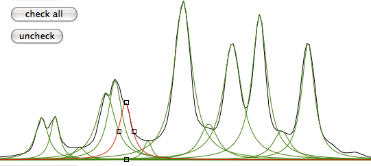
You start selecting a region of a 1D spectrum, already completely processed. The command "Deconvolution" creates the window shown in the first picture. In normal circumstances we'd enlarge the window as much as we like. For the sake of readability of this blog, we keep it small. You can see the experimental spectrum in black and the peaks already fitted (in a very approximative way) with green lorentzian shapes. The selected peak, in red, has a shoulder on the right, but only in the experimental spectrum. To create it in the simulated spectrum too, first we split the peak in two. The leftmost icon performs this operation on the selected peak.

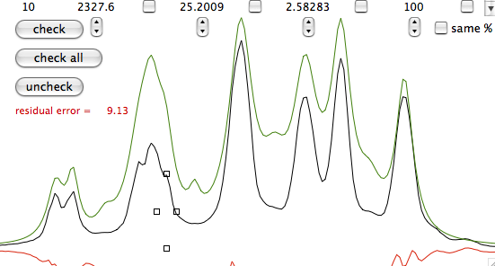
The second picture shows the two halves, red on the right. green on the left. By dragging the square black handles, we can manually fit the peak and the shoulder (see below).

It's now necessary to observe our data differently. With the command "toggle", the green shape corresponds to the sum of the peaks (i.e. the simulated spectrum), while the red line corresponds to the difference (experimental - simulated).

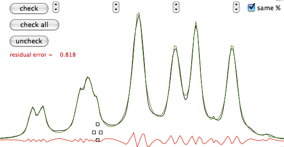
Manual fitting is out of question. Before performing automatic fitting, we have to specify which parameter should be changed. In this case, a click on the button "check all" selects all parameters for adjustment. Another click on the heart icon and we arrive at the last picture.

Summary: iNMR specifies the initial parameters, but you can add or remove peaks, shift and reshape them. You have a table at the top if you prefer a numerical input. In this way you can specify: position, shape (lorentzian, gaussian or anything in between), area and width for each line. Graphically you specify: position, height and width. You can mix manual and automatic fitting, the former extended to all parameters or only to selected ones. You can optionally specify that all peaks are described by the same function.
Eventually you get a good estimate of all parameters (e.g.: area, position...) for each peak, even the hidden ones.