Monday, June 30, 2008

Selective Attenuation

We can alter the FID at our advantage. It's enough to multiply the complex FID with a positive real function. Many functions have been proposed and it's difficult to find other common properties among them. Most have zero intensity at the end, but there are also exceptions. To do something useful with these functions you must be aware of your particular needs. Think in terms of: "What do I want to attenuate?". The name "Weighting" only describes the "how". A description of the "why?" would be: "Selective Attenuation". I have counted 4 things that can be attenuated.

1) NOISE
After multiplication with a negative exponential (2 Hz) this spectrum becomes:


2) LORENTZIAN TAILS
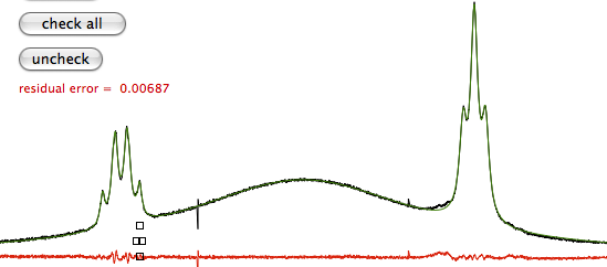
The tails of NMR peaks are much larger than you may think. The components of a multiplet are often fused into a single group. In this case, the apparent distance of two positive Lorentzian curves is less than the actual distance. I can attenuate the tails and obtain a complete separation of the above signals with a positive exponential (1.6 Hz) and a gaussian (1.2 Hz).


3) DISPERSION TAILS
When a spectrum is in magnitude or power representation, you have a mix of absorption and dispersion curves. The latter contribute with large and nasty tails. I have attenuated them with a sine bell shifted by 6º.


4) TRUNCATION WIGGLES
This synthetic FID does not decay. I can attenuate the wiggles (without generating tails) with a cosine squared function.


Do you know about other things that can be selectively attenuated?

Saturday, June 28, 2008

Success

With my great surprise, the number of visits to this blog reached a peak yesterday: 95. While the number in itself is still miserable, the average is even worse: 65. It's a mystery why I have attracted the highest number of visitors the day I had less things to say.

If the picture was the cause of such a success, let me try it again. It's the same subject in Leopard style.
I have added new links into the sidebar.

Friday, June 27, 2008

Interlude

It's not elegant to start a new topic on Friday. Before tackling new difficult concepts, an interview is more relaxing. In almost two years of blogging, this is our first interview, and a special one, with my alter ego Giuseppe Balacco, author of iNMR (the name says it all). I meet Giuseppe in a hot summer afternoon. He is sweating into his hot room, watching at the quotes of the stocks on the monitor and listening to one of his records. The first questions are almost instinctive.
Q. Are you monitoring your stocks?
A. I only had €10K invested, for 3 months. I sold everything one month ago, with a gain of 300, more or less. I am lucky that I have no money to invest, because these prices are too luring to resist. Actually I suspect that stocks are, still, way too overpriced, and they will keep falling for a long time. Italian stocks at least can keep falling for another couple of years: there's no parachute. It's funny to watch these movements, because they are unpredictable. Look at Buzzi Unicem: the ordinary stock goes up +1.13%, while the preferred stock goes down -0.93%. It's the same company, isn't it funny? It's also funny to compare the movements with the forecasts! Well, I know, this time should be invested into real work, instead of speculation; actually I am doing nothing at all, it's too hot for any kind of activity! I am more inclined to philosophy. These continuos movements of money are the symbol of the world we live into: every day we are exploited by banks and speculators.
Q. What's the name of the record you are playing?
A. "From the Hot Afternoon", by Paul Desmond. It's an atypical pop effort by him. I prefer his solo records over what he did with the David Brubeck quartet, because I dislike Brubeck. "Take Five" is the exception that proves the rule. Unfortunately Desmond had little time to make records under his own name. According to the established classifications, he should be the quintessence of cool. Do you feel the cool?
Q. May I have a glass of ice-cool water, please? Let's talk about your product. Why have you changed the package of iNMR?
A. It all started on the Firefox Download Day. We were sitting on the sofa, watching the football match (yes, the European Championship), and my daughter was, at the same time, surfing the internet with her laptop. We began talking about what she was doing and then I saw her installing Firefox. I liked that minimalistic blue background and I said to myself: "Copy that style".

Q. Were you tired of the old background? Wasn't it more spectroscopic?
A. The old background was nice, otherwise it wouldn't have lasted almost 3 years. It was too baroque, but that's good because I like the baroque style. The fact is that, initially the icon of iNMR derived by the old icon of SwaN-MR. In 2006 a new icon was introduced, but the background wasn't changed; it had to be. It was a little too heavy, I mean it weighted 140 KB, while the new one is only 36 KB. Let's save a little of bandwidth, why not?
Q. It's also more in line with what Mac users expects nowadays?
A. Yes, this new kind of packages, with the huge Application folder alias, emerged in 2005, the same year that marked the appearance of iNMR. I should have adopted it earlier, but there were different priorities. My policy is to follow the directions given by the users and nobody had never asked for a different package, nor did anybody found it difficult to install the evaluation copy. They have been keeping asking for a lot of changes, but nobody complained about the package.
Q. I have noted that your policy about evaluation copies is to limit their functionality, rather than setting a time limit.
A. That sounds obvious to me. If you had evaluated iNMR in 2006, then in 2007 and then again today, you would have found a lot of new things each time. Look at the list of recent changes. This one covers the last 17 months only, the whole list would be longer! I wanted people to be able to try all of the additions, as they were appearing. And, obviously, with no expiration date there is one thing less to decide: how long should the evaluation period last? Every user has different needs. 1 day can be enough and 1 year can be not. Last, but not least, I myself am using other programs in evaluation mode. Take, for example, the blue background of the new package. I made it with WouldjaDraw, a program that can be used for free 20 times, before you have to pay. Up to now I made two pictures (in 2 years). I know that a similar thing happens with iNMR. If you only need it once a year, and you don't need to print anything, you can use it in evaluation mode, and pay nothing. You can also use it every day, it's perfectly legal, but at this stage people prefer to become regular customers. There are too many advantages, compared to the price to pay.

At this point Giuseppe saw I was tired and offered an ice-cream. We spent the rest of the time listening to Paul Desmond. Soon or later I will return to his room with a camera, for a full reportage...

Thursday, June 26, 2008

Frontier

I have no experience with line-fitting in 2-D and 3D spectra. I have never studied it and don't know what people have already done and which is the current approach. This is a blog and I want to use it like a blog, to express my ideas. I hope you'll also want to treat it like a blog, not as a textbook. If one day I am going to put my hands into this matter, my ideas will certainly evolve, as it always has been when passing from planning to real problem-solving.
nD spectra are more problematic than 1D spectra:
  1. There are more parameters to estimate (the double in 2D and the triple in 3D).
  2. There are less experimental points.
  3. The shape is not Lorentzian, because the FID is multiplied by weighting functions.

A direct solution is to simulate the FID with exponentially damped sinusoids, apply the same weighting that has been applied to the spectrum, and compare the synthetic spectrum with the real counterpart. The fitting algorithms, alas, require the partial derivatives. I can't know their analytical formula (the weighting functions are not know at compile time, and even if they were...), but I can simply use the ratio Δf(x)/Δp, where f(x) is the spectrum and p the parameter. This direct solution requires more experimental points that is common to find. Requires quite a lot of programmatic work. It's purely computational, while I like interactive adjustments, where the user can manually change the parameters at any stage through a GUI.
Alternatively, I would start approximating. I'd assume, first, that the signal has not decayed too much or that the peaks have similar widths, therefore the shapes are common to all peaks (they would mostly depends on the weighting functions that have been applied, but it doesn't matter a lot). Second assumption: the common shape can be adequately approximated with a mixed Lorentzian/Gaussian function, namely:
f(ν,δ,I) = α L(ν,δ,I) + (1-α) G(ν,δ,I)
where 0 ≤ α ≤ 1, ν is the central frequency, δ the line-width at half height, I the area. Many peak shapes can be approximated with this formula. With this approach, The number of parameters decreases, because all the peaks would have the same δ and α along f₁ and another couple of shared values along f₂.
That could work, but: who needs it?
Here's a practical case: a ROESY with weak cross-peaks. They are dominated or polluted by DQF-like cross peaks that not only hinder the normal integration process, but are typically sharper than the genuine peaks, therefore my model can't work (not all the peaks have the same shape).

Wednesday, June 25, 2008

Blindly

In the last few days I have been giving the impression that line-fitting is much more time-consuming, difficult and error-prone than integration. It's true, not because line-fitting is more complicated, but because integration is simpler. There are also notable exceptions. The last tutorial published on www.inmr.net illustrates the case. Here is the spectrum to "integrate":
It's the kinetic study of a chemical reaction. Not only the concentrations change, but also the frequencies. That's not at all a problem. If you give a look at the article, you see that it's possible to measure the concentrations of all the diagnostic peaks in all the spectra with a single operations. In other words the whole job, including the formatted table of the estimated areas, can be done by the computer in automatic fashion.
In this case, they exploit that fact that line-fitting not only gives the intenisities, but the frequencies too. In this way it's easy for the computer to drift along the ppm scale without error. Actually, there are a few, unavoidable, errors, when the computer attempts to measure the concentration of the product at the beginning of the reaction. Examining the bottom spectrum visually, for example at 5 and 11 ppm, I can't even tell where is the peak. In such a case I think that deconvolution is too risky to rely upon it. It is better to integrate a frequency region large enough to contain the peak, even if I don't know its exact position, to measure an adjacent and transparent region of the same width, then to calculate the difference. The cumulative error can still be quite high.
Yesterday I dispensed a lot of strategies for line-fitting, today I am showing that you can do it blindly. Both things are true at the same time. In today's case, the operator first performed the process manually on one of the spectra, then wrote down a macro to extend the treatment to the whole experiment. Apart the very first spectra where the product is invisible, the rest of the task is easy. There are mostly doublets or singlets. (Connecting to my Monday's post: why using the term "deconvolution" in such a case, when the purpose is merely to remove the noise, not to remove the broadening?).
Furthermore, there is so much information available (a whole matrix of correlated values) that you can't be obsessed by the fear of errors. If there is an error, it is easily spotted. Different is the case when you have a single spectrum to process and you can't even find a denomination for the multiplet structure.
A proton spectrum or the altimetric outline of a dolomitic stage at the Giro?

What I am going to opinionate now it's not specific to deconvolutions, but applies equally well to integration. We are so used to equate the integral with the concentration that are tempted to make the big mistake of comparing the integrals of two different spectra. Even when the sample tube has not been extracted from the probe and the acquisition parameters are exactly the same, it's not always a safe practice to assume that the concentrations are proportional to the integrals. That's what we do to measure the relaxation times, and it's OK, because, in that case, less accuracy is tolerated. When studying a kinetic we can, and therefore should, use an immutable peak as a concentration standard. If the immutable peak is not available, or even when it is, we can start from the integrals to measure the percentages of the two compounds (starting and final). In this case, if we assume that there is no degradation to a by-product, the total concentration is constant and the percentage values are proportional to the single concentrations. In other words, the percentages are internally normalized and therefore comparable between different spectra. It doesn't represent an extra workload, because it is easily done inside Excel, and you are going to use an Excel-like program in any case.

Tuesday, June 24, 2008

Factorize!

Yesterday I introduced the subject of curve-fitting. Today we'll examine the practical details.
A computer can do breathtaking things, like finding out 10 parameters in less than 1 seconds. If you rely too much on it, however, you will be often disappointed. Treat it like a thoroughbred and the computer will serve you faithfully. The first principle is to split any problem in parts. Although you can build a model that accounts for phase and baseline distortions, that's a wrong strategy. Spend all the time required for professional phase- and baseline- corrections. Then start assuming that your spectrum only contains lorentzian peaks.
You also have the precious weapon of gaussian lineshapes. They are not a natural shape into NMR spectra, therefore use them as little as possible. There are programs able to search for the optimal mix of functions. You can try this option too (when noise is moderate). Normally the result will be > 90% Lorentzian. When it happens, stick to purely Lorentzian shapes.
Before the game begins, you choose the battlefield, that is the portion(s) of the spectrum to fit. The number of experimental points must be higher than the number of parameters to fit. This can be a problem in 2D/3D spectroscopy. In the 1D case it's rarely a problem. Pick only the central part of the peak, that emerges from noise.
If the peaks nearby are weak, in comparison, don't include them or their tails into the battlefield. If you include them you also have to fit them. (Remember our motto: "Factorize!"). Into the picture I have highlighted the portion of the spectrum I'd sample to fit the central doublet. It's true that a Lorentzian curve has long tails, but it's not necessary to select them. If the magnetic field is not homogeneous, the tails are actually deleterious, because they deviate from the theoretical shape.
The fitting process doesn't start from vacuum. You have to declare the number of peaks and their tentative parameters. The computer itself can do it for you, but that's the part that humans do better. The frequencies are easy to guess, both for you and the computer. If you set them with care, you can be more vague with the remaining parameters. Anyway, the two operations (sensible guess and least-squares fit) can be repeated and mixed at will. After a fitting run, you can modify some parameters and try again. In the process, you can decide that a parameter can't be further optimized (often the frequency) and freeze the corresponding value. If the value is correct, there will be more chances of success (if it's not correct... more chances of failure).
The least-squares algorithm converges into a local minimum, often but not necessarily the nearest one. A systematic grid search could probably find the absolute minimum, but it doesn't look like a sensible strategy. Most spectroscopists extract the NMR parameters without even knowing the word deconvolution, therefore you should be able to furnish a starting guess that's good enough and whose nearest minimum is also the global minimum. Everything can be done within the GUI: the definition of this starting guess is a graphic process, as simple as drawing a formula with ChemDraw.
You may think that with a suitable linear combination of many lorentzian and gaussian curves you can fit any mountain. That's almost true, but the computer might disagree. For example, if the experimental spectrum to fit only contains a single asymmetric peak and the starting guess is a doublet, during the fitting process the intensity of one of the model curves might go to zero. It means that the computer has decided that the peak is unique and nothing can change its mind. This is not a rule, you can often simulate a shoulder by declaring a small additional peak. If the program tends to cancel it, you can fix the parameters of the shoulder (set them manually and remove from the fitting). It is equivalent to subtracting the shoulder from the experimental peak and performing the deconvolution on the difference spectrum.
You may be tempted to define relations between the parameters. A trivial example is to keep equal the intensities of the two components of a doublet. Don't forget the roof effect or, in more general cases, quantum-mechanical effects. In such a case, instead of fitting the spectrum against a set of curves, fit it directly against a whole spin system. The problem is akin, but more specialized tools are implemented. I'll touch them sometime in future, but there is still another couple of things to say about curve-fitting. Tomorrow.

Monday, June 23, 2008

The Name of the Game

Waves are only one kind of the shapes we can fit. In time domain we only have waves. In frequency domain the variety of shapes is higher. Peaks can be well approximated with Lorentzian curves, but in rare cases an anomalous spike can be better fitted with a Gaussian curve or a combination of the two kinds. Weighted FIDs generates all kinds of shapes, presumably. Another familiar profile is the dispersion Lorentzian curve, which also has its own math expression. In theory anything can be fitted by an HIGH degree polynomial, but in practice that is only appropriate for the baseline.
Fitting the experiment to a model is a general procedure that goes well outside the world of NMR. In our little world it is commonly called "deconvolution". Is it the same outside? While this is a word with a gentle sound, and I like using single words instead of long expressions, I think that the name is not appropriate, also because deconvolution has its own meaning and math expression. When you add a line broadening factor to a noisy 13-C spectrum, you are actually convoluting the existing peaks with a Lorentzian shape. If the line broadening factor is negative, you perform, de facto, a deconvolution. My readers are able to find all the good reasons to explain why we call deconvolution what should be actually called line-fitting and weighting what should be called (de-)convolution, and I don't argue. I also dislike the sound of the word "fit". In the following I will freely use both terms. You know what I mean.
This is one of the funniest things in NMR processing, for two reasons: first, it frees the spectrum from noise; second, it is not trivial, therefore achieving a good fit is always a cause of joy and satisfaction. In practice it only lasts a few seconds and the victory is almost certain; it's a video-game with a little less fun and much less stress. I am aware that deconvolution can be performed by the computer in an unattended way, yet I tend to believe that success requires strategy, experience, tactic, patience, luck, self-esteem and ingenuity (all in minimal doses).
The computer measures the goodness of the fit by the residual quadratic error; the user relies both on this value and on the similarity of the two plots (the spectrum and the model). There is nothing sacred in neither measure. They are only two details and I look to the whole picture. The numbers you get by line-fitting are always to be compared to other numbers. For example, you want to compare the concentrations of a metabolite in different samples. You can judge by yourself if the variations make sense, but you can also compare your concentrations with the literature values, or the values found by another analytical technique, or the values found fitting a different peak of the same molecule, etc...
There is the statistic-kind of analysis, the so-called error analysis. I agree that some games can be boring, but statistic is way too dull! (The dullest discipline I have ever come in contact with). If it only yielded meaningful numbers, I would happily tolerate it. When I have found or calculated those confidence ranges, I have seldom found them worthy of any confidence. Probably the theory of error analysis doesn't apply to NMR (the single points aren't independent observations, the errors aren't distributed normally, etc...) or, more simply, I couldn't find anybody willing to teach applied statistic to me.
I am going disclose my secret strategies tomorrow. Before closing the post, I want to pass the concept that deconvolution is not a better method than integration in all circumstances. While accurate integration already has its requirement (complete relaxation between scans, flat baseline), deconvolution also requires good magnetic homogeneity, and elevate digitization. Integration is affected by noise in a limited way (and when the noise is much higher than the signal there's no method that works). The advantages of deconvolution are that you can measure the ares of overlapping peaks, but also the frequencies and the linewidths.picture taken from www.inmr.net

Friday, June 20, 2008

Looking Back

Several methods have been proposed to calculate the LP coefficients; the fact that no clear winner has emerged demonstrates that it's a tricky task. My choice was casual. I remember being into the library (it was probably 1991), browsing the latest issue of a chemistry journal (don't remember which) where I probably I read the expression "Linear Prediction" for the first time in my life. What I remember with certainty are the names of the author: Gesmar and Led. They were discussing the application of a novel algorithm ("Fast Linear Prediction"). Curious to see it in action, I wrote to the duo asking for the source code. They replied that the code was available for sale, and the price resulted to be higher than my monthly salary. What they were selling in practice was the FORTRAN source code of a program written for the VAX. A program with a single routine. I had no FORTRAN compiler, no VAX machine and no idea about a practical application of LP that could justify the expense. Now, being that the algorithm had been invented by someone else, a mathematician called George Cybenko, I wrote to the latter. Unfortunately, during that period he was recovering from a broken leg (skiing). When he returned to work, after months, he sent a fax. From that moment on, he began collaborating with me and, fax after fax, helped me in writing his algorithm into my language (during the period I had a Pascal compiler). I spent a lot of time first to understand the algorithm, then to write it, finally to optimize it for speed on my computer. Enough reasons to remain affectionate and faithful to it for years, yet now I almost convinced it represents a second choice.
Do you remember the synthetic spectra I used to demonstrate the properties of zero-filling? It contains 10 exponentially decaying sinusoids, with identical line-widths, not-too-different intensities and spread-out frequencies. I have used Cybenko's algorithm to calculate 10 prediction coefficients; then I have told the computer to prolong the FID using the coefficients. The synthetic FID is perfect:The part at the right of the vertical red line has been predicted correctly. So far, so good. All of a sudden, if I repeat the calculation with 11 coefficients instead of 10, it's a disaster:

This time there is no necessity for the red line! What's the cause of the disaster? The lack of noise! When there is a minimal amount of noise, it can neutralize the excessive number of coefficients. When the number of coefficients grows further (e.g. > 40) the disaster is almost guaranteed, however, there's no excuse. I avoid using this algorithm with more than 24 coefficients. The alternative is to use a generic algorithm, therefore slower, to solve the same system of equations. A popular algorithm, probably the most popular method of Linear Algebra, is the singular value decomposition. With SVD I get the same perfect results if I calculate 10, 11 or even 100 coefficients. There's more. I also get the ordered list of the so-called singular values. For example, if I ask the computer to compute 20 LP coefficients, it can also give me the following singular values:

01 227399.55548
02 212850.09660
03 208405.44529
04 171681.01548
05 154987.64513
06 120658.53137
07 104391.19112
08 99881.44088
09 83773.77349
10 64064.17610
11 0.00547
12 0.00540
13 0.00536
14 0.00535
15 0.00532
16 0.00527
17 0.00519
18 0.00512
19 0.00503
20 0.00500

I have not explained what a singular value is because I am an ignorant. Even an ignorant, however, understands that SVD offers the welcome bonus of measuring the number of signals contained into an unknown FID. A useful option of SVD is that the computer, after having detected that the nature of the problem can be better described by a smaller number of values, can ignore the rest. This option is ON by default. I supposed that this self-regulation was the cause of the stability of SVD. I wanted to verify what happens if I disabled the option. Surprise: nothing changes! (and nothing remains for me to speculate about).
From this single, unrepresentative test, it's clear that SVD is far better, but I haven't the slightest idea why. (For completeness: SVD can cut down the number of singular values, but not the number of LP coefficients; this is something you need to do on your own).
There are also abundant methods to save the day when the coefficients don't work, and they don't depend on how you have extracted them. When I introduced my "theory" of LP, two days ago, I explained that the LP coefficients of the isolated signals (related to the frequency and line-width) are different from the LP coefficients of the full spectrum, but can be recalculated from the latter. It's enough... (!) to solve a single equation of the nth degree (where n is the number of coefficients). Assuming that the task is simple, when you have the roots of the equation, you can verify the only condition we know: the ratio α = I₂ / I₁ must be < 1 in the case of forward LP and > 1 in the case of backward LP. (Cfg. my old post for the meaning of the symbols).
Everybody agrees on this point. No theory, unfortunately, says what we should do when the condition is not verified (and it happens incredibly often!). In the case of forward LP it is possible to substitute α with its reciprocal. The consequence is that the FID decays even faster than it would do naturally. The result is an hybrid between LP and zero-filling, and it can't be harmful. In the case of backward LP, instead, the same trick will make the FID grow (backward) more than it ought to do, with invariably catastrophic results.
That's why I prefer forward LP.

Thursday, June 19, 2008

Looking Forward


The polygons are the idealized shapes of the FIDs of dioxane (green) and water (red). We suppose that the magnetization of water decays much faster, just to see what could happen in extreme cases. We also assume that, when the signal decays under a certain level, it has no more effect on the detector (in other words, it's zero). In both FIDs the evolution of the signal can be summarized with a single parameter, given by the ratio of any two contiguous points. They can be taken from the beginning or the end of the FID, it's just the same. Once we have the prediction parameter, we can prolong the FID indefinitely. (In the red case, there's no difference between forward linear prediction and zero-filling).
Now let's mix dioxane and water:


As explained yesterday, now we need 4 contiguous points at least to extract the two prediction coefficients. We can't choose them from the beginning of the FID (dominated by the water signal) because there is no more water in the portion of the FID we are going to predict. We must choose the final points. The lesson is: calculate the prediction coefficient from the same end of the FID you are going to prolong. Now let's consider another signal (tangerine) in the presence of noise (gray). Noise doesn't decay.


In this case it would be more convenient to exploit the initial points of the FID, because there is less noise (in percentage) and the estimated parameter will be more accurate. That would go against the only rule we imposed to ourselves a few lines above. To reduce the effect of the noise we can, however, make use of the whole FID. This can't be a rule. Sometimes you can see by inspection that a portion of the FID is irregular. Ever seen a FID coming from an Avance instrument? The very first points aren't useful for linear prediction.
In a fourth case we consider a spectrum with very little noise and a signal that decays to undetectable levels:


Most of the proton spectra acquired today correspond to this case. If we use the whole FID, we can calculate the coefficients with accuracy. When we prolong the FID, all we can prolong is, however, noise, because the true signal is already negligible at the end of the FID. The good thing is that the predicted noise will soon decays to zero (at the same rate of the blue signal); but zero-filling is even better, because it decays immediately!

LP is slower and less stable than FT. We had an hint yesterday. The formula to calculate the complex prediction coefficient would be:
p = S₂ / S₁.
Of the 4 arithmetic operations, when performed on a computer, division is the slowest and the less stable one. The formula for the FT contains a multiplication and an integral (that is, a sum), but no division.
Another inherent weakness of LP is the propagation of inaccuracy. Each point is predicted according to what comes before. The first point you predict is based exclusively on experimental data. The second point is also based on the first point, which is artificial. The third point is also based on the second point, a second generation artificial point. The 1001th point is also based on a 1000th generation artificial point. If there was a defect of precision, it has been amplified 1000 times.
If the last part of the experimental FID is dominated by noise, you risk to amplify it thousands of times.
In practice things aren't so bad. There is a single case I know when forward LP is useful. It's when you want to prolong the indirect dimension of a 2D/3D spectrum. Let's say your 2D spectrum requires 2 days of spectrometer time. You can decide to truncate it after 12 or 24 hours and predict the rest. From our discussions you can deduce the requirements: the number of points (in the indirect dimension) must be at least twice the number of signals (for the most populated column), the signals haven't decayed too much, noise should be low. The conditions are easily met in ethero-nuclear 2D (only a few cross-peaks per column; in the case of HSQC of small molecules they are 1 or 2). In the homo- case signals, when are much more, forward LP is often beneficial too. Evidently, it can work.
Next time we'll unleash the algorithms.

Wednesday, June 18, 2008

Clockwork

Consider a sample of pure water, with a single NMR resonance. After we excite it, we have created a magnetization vector that rotates into the xy plane. We observe the magnetization at regular intervals. The show soon becomes dull and repetitive. Actually, after the first two observation, we can already predict all the remaining ones. Let Φ₁ be the phase observed initially, and Φ₂ the next sampled phase. We can calculate:
Δ = Φ₂ - Φ₁.
Δ remains the same for every couple of consecutive observations. For example, we can predict:
Φ₃ = Φ₂ + Δ.
Φ₄ = Φ₃ + Δ.
Because the intervals are all equal. The value of Δ must be related to the frequency of the signal, of course, but we need not to know neither the relation nor the frequency.
There's a difference between the magnetization vector and the hands of a clock: the former is subject to exponential decay. After we have measured the intensity of the magnetization twice, let I₁ and I₂ be the two values, we can calculate:
α = I₂ / I₁.
α must be < 1, because I₂ < I₁, otherwise it's not a decay. It's also α > 0, because we are considering the absolute intensities here.
If the decay is exponential, we can predict:
I₃ = α ⋅ I₂.
I₄ = α ⋅ I₃.
The value of α must be related to the relaxation time of the magnetization and the broadness of the signal, of course, but we need not to know neither the relation nor the broadness.
Phase and intensity can be observed simultaneously. If we observe the magnetization twice, we can completely predict its future. Remember this number 2. The number of observations must be at least twice the number of signals. Information about phase and intensity can be stored into a single complex value:
S₁ = I₁ cos Φ₁ + i I₁ sin Φ₁.
α and I can be similarly stored into a single complex number p, called prediction coefficient. The number of coefficients must be at least equal to the number of signals.
p = α cos Δ + i α sin Δ.
S₂ = p ⋅ S₁.
S₃ = p ⋅ S₂.
Instead of water, we may have dioxane, with different frequency and relaxation time, therefore a different prediction coefficient q:
q = α' cos Δ' + i α' sin Δ'.
Finally, let's mix water and dioxane. The spectrum will be a sum of predictable spectra, therefore itself predictable. When there are 2 signals, we need 4 observations S₁, S₁, S₃ and S₄. Using them, let's write down a system of equations:
S₃ = x ⋅ S₂ + y ⋅ S₁.
S₄ = x ⋅ S₃ + y ⋅ S₂.
There is no need to explain the above equations. They are the definitions of two new coefficients x and y. You don't demonstrate a definition. If we solve the system of equations, we also know the values of x and y. They predict all the future points. For example:
S₅ = x ⋅ S₄ + y ⋅ S₃.
This is forward linear prediction. Backward prediction is specular (Δ changes sign and α becomes its own reciprocal). We assume that 2 coefficients are enough, because the complexity of the problem is proportional to the number of our signals. It's not forbidden to define more coefficients than necessary, the prediction will still work.
x and y are related to the coefficients p and q of the isolated signals. For completeness:
x = p + q.
y = - p ⋅ q.
When you have more than 2 signals, even hundreds of them, build a polynomial an solve for its roots. The order of the polynomial is equal to the number of signals. For example:
z² - xz - y = (z - p) (z - q) = 0.
In theory, all we have seen is valid. Tomorrow we'll follow an empirical approach.

Tuesday, June 17, 2008

Nothing Is Better

A few months ago I commented on zero-filling on Glenn Facey's blog. I have reordered my own comments and here they are. In the following I mention Linear Prediction (LP). It's a technique I am going to explain tomorrow.

"Maybe a few readers of this blog, less fond of math, can better understand the following simple recipe. In high resolution 1D NMR, usually the signal has already decayed to (practically) zero at the end of the FID. In this case zero-filling and forward Linear Prediction should yield the same results, but the former is better (faster and more robust). When, for whichever reason, the signal is truncated, the preference goes instead to LP.

The statement "it is only forward linear prediction which adds new information to the spectrum" is not correct.
1. LP can't add any authentically NEW information because it simply extrapolates the information already contained into the FID.
2. Zero-filling has the property to recover the information contained into the imaginary part of the FID (uncorrelated to the real part) and to reverse this additional information onto the real part of the spectrum.
(see demonstration below)
3. The spectroscopist, to run an LP algorithm, feeds it with the hypothetical number of lines. While this is certainly NEW information not already present into the FID, it is arbitrary.
Bottom Line: LP is a good thing, yet things are more complicated.

DEMONSTRATION (?!?)
Let's say you collect a FID of n complex points. It's a sequence of n real and n imaginary numbers or measures. They are independent measures, because no single value has been calculated from the rest. The total information content of the experiment amounts to 2n measures. After FT and phase correction you have a real spectrum of n points while the imaginary spectrum is discarded. You may ask: "Why are we throwing away half of the information?". We could rescue it with an Hilbert transform (HT). It's a tool to calculate the imaginary spectrum when you only have the real part, or the real spectrum when you only have the imaginary part. If the noise of the imaginary part is uncorrelated to the noise of the real part we can add:
experimental real spectrum +
real spectrum regenerated from the imaginary part =
more signal/noise.
The HT works in this way: you set the real part to zero, apply an inverse FT. You reach an artificial FID which is (anti?-)symmetric (both the real and imaginary parts first decay, then grow again). Set the right half of the artificial FID to zero, then apply a direct FT. (I have omitted the adjustment of intensities, because I only want to show the concept).
As you can see, HT is akin to zero-filling. Although this is not a mathematical demonstration, it may convince you that zero-filling can move some information from the imaginary part onto the real one, so can enrich the latter with real information.
It only works, however, when the signal has already decayed to zero at the end of the FID, otherwise it's so unrealistic that generates unwelcome wiggles."
Here I wrote: "I am sorry I can't find a literature reference with the real demonstration".
Mike kindly added:
"I believe that the reference old swan refers to is a paper from Ernst's lab: JMR, 1973, 11, 9-19"

NOTE
When I commented on Glenn's blog, I wrote that the artificial FID, intermediate stage of the Hilbert Transform, is symmetric. This is the graphical impression. But, who can recognize if the sign of the FID changes? It looks just the same; (unless the oscillation is terribly slow, the envelope remains the same). This is a detail that doesn't affect at all the rest of the discussion. We are going to set to zero the second half of the imaginary FID, so it doesn't matter which sign it has before. The book Numerical Recipes contains a correspondence table (page 601 on the 3rd edition) between symmetries in the two domains. From the table I understand that, in our case (real spectrum = 0), the real FID is odd and the imaginary FID is even.

Monday, June 16, 2008

Size Does Not Matter

Zero-filling can't be dangerous. Here is the practical demonstration. I have created an artificial FID with 10 ideal signals (decaying exponentials).

All the signals have the same widths and all are truncated. If I apply zero-filling from the original 4096 points up to 32,000, the spectrum shows bad-looking wiggles.

If you only look at this picture, it seems that zero-filing is a cause of problems. It is true that, without zero-filling, there would be no wiggles. Let's try to FT the original 4096 points directly:

Hear: this spectrum is perfectly phased. When I have created the FID, the waves were all in phase. The experiment demonstrates that truncation causes an asymmetric shape change. Zero-filling, if applied to a truncated spectrum, restores the symmetry (beneficial effect) but at the cost of introducing wiggles (side effect).
black: truncated FID + FT
red: truncated FID + zero-filling + FT

Zero-filling is not responsible for the truncation. It has stressed in a special way a problem that was already there. If there is no truncation, a zero-filled spectrum can only look better than the original. If there is truncation you should resort to a longer acquisition time (if you can) or to Linear Prediction (in the remaining cases).
With today software you can monitor the effect of zero-filling on the fly (in 1D at least). It's enough to select a new value and the spectrum is instantaneously updated. If you see no difference, reselect the old value. I can see a severe effect when I truncate the spectrum, but when I increase the size it's hard to see any difference on the monitor. What I see is that, the bigger is the size, the slower is the computer. Just because I like to experiment with all the other real-time manipulations available (weighting, phase and baseline correction, etc..) I think it's better to zero-fill afterwards, after I have already decided/found the remaining processing parameters (but before performing peak-picking). This is the advantage of using a computer: you don't have to set the parameters in the order they are used by the program. You can set the parameters in any order at any time. It is necessary, of course, to reprocess the spectrum, but it usually takes less than 1 second. If it took 1 hour, than there would be an advantage in being an expert and knowing the optimal parameters in advance. But processing is thousands of times faster and the true advantage is when you don't take anything for granted but are curious enough to experiment.
An high number of points is required when you want to study the shape of the peaks or something related to it (for example, if you want to fit your spectrum with a simulation, for whichever reason) or when you want to measure coupling constants with accuracy. If I am aware of such a need before acquiring the spectrum, I don't rely on zero-filling but prolong the acquisition time.
Everybody can verify that extensive zero-filling has no visible effect on a properly acquired spectrum. Why, then, spending time with interactive optimization? Can't we adopt a rule and stick to it? Yes, it is known that the optimal zero-filling doubles the size of the FID. I remembered that the demonstration dated back to the early days of FT-NMR but could not find it again. The reference was kindly found by Mike:
JMR, 1973, 11, 9-19
This story will be the subject of my next post.

Saturday, June 14, 2008

2D Plot

When I am tired of sitting in front of the computer, I have two options. If I go to the countryside, I see litter along the roads, and that's not an inspiring sight. If I go to the harbor, it's more romantic, thanks to the water that covers and hides what's below. I know that there can be plenty of litter under there, but it's invisible and I enjoy the scenery. In NMR spectroscopy, 1D plots are the countryside, where you are forced to see the noise, 2D plots are the seaside. When I was a beginner, I was tempted to dry the sea to observe the hidden treasures. I found none. There's only litter at the bottom. Now the level of my spectroscopic sea is sensibly higher, but I am still the master of the tide and keep playing with it.
The computer programs are obsessed with the idea of expressing the intensity of the signals through color. I have already discussed this point in the past. There are two kinds of plots to consider. One is the bitmap or fast plot (like a photo), the other is the contour plot (like an ink drawing). In the first case you can have an (almost) continuous gradation of hues. I only use the bitmap for processing and I don't care too much about the colors. All I ask is that positive and negative peaks are well differentiated.
The contour plot, though slower and less informative, is more synthetic and, therefore, readable. I can both raise the tide from below and truncate the mountains from the top, remaining with only the shape of the islands. Most of the times, I keep 9 positive levels and 3 negative levels, in geometric progression (factor = 1.4).
I try to be as consistent as possible, while the programs encourage customization and babelization. You may find it funny to print a plot in 24 colors, I find it unreadable.
With 4 colors you can show everything:
1 dark color for positive islands;
1 dark color for negative islands;
1 light color for positive cliffs;
1 light color for negative cliffs.
Two colors (after raising the tide and burying the cliffs) are even better.
While, in 1D, it's difficult to realize that points have a finite size, it's natural in 2D to realize that a point is actually a small tile. Graphic cards are also optimized to reproduce bitmaps. Bottom line: drawing a 2D spectrum is less problematic.

Friday, June 13, 2008

1D Plot

Drawing a spectrum is not the most stupid thing a computer can do. Actually it requires a lot of patience and dedication, both for a programmer and a user. All the computer has to do, in the case of a 1D spectrum, is to connect adjacent points. They are also equally spaced, along the x axis. Where's the complication? Furthermore, little has changed in the last 20 years. The only change I notice is that there are less plotters around today, which means more room in the lab, less machines to maintain and less drawing routines into the program.
Unfortunately computers seems to follow the Murphy's law: they always find a way to complicate my life. I told you that I installed Jeol Delta, courtesy of Jeol, but it's too difficult for me to use. It draws spectra wonderfully, into a small pane, and I don't know how to enlarge it (I'd like to see the plot as large as my monitor). That's not a big issue, because Delta would still remain too complicated for me to use it. I also have Mnova, and I know how to use it. Mnova can draw a plot as large as the window, but it's painfully slow. I have tried to modify the settings, and actually the situation improves a lot with the option "Entire Page" and the pen width = 1. Even after this optimization, Mnova still remains slower than Delta. With the latter I can continuously change the intensity of the spectrum, and the response is fluid. Mnova reacts very slowly, instead, showing a flashing watch cursor, whenever I roll the scrolling wheel. Surprisingly, the manual phase correction appears more fluid (the computer is doing the same things plus additional processing, yet it takes less time! why?). In conclusion, I have discovered how to make the plot as large as the window, but it's impossibly slow, therefore I have switched to the "Entire Page" mode, which is uncomfortably slow.
For me the drawing speed is fundamental, because I navigate a lot through my spectra and want the computer to be as fast as my hands. There are, also, economical and psychological motivations: I expect any new combination computer+software to be as fast as its predecessor. I assume that the fault is mine or of my computer, but what can be good news for you is bad news for me (if the problem was more generalized, I had some hope to find some help some where). Don't worry about me, I also have a third program that combines the largest size with the fastest speed; I dubbed it "the ultimate NMR experience".
Today's graphic cards can be faster than the rest of the machine, but only when they like, and they have never learned how to draw a 1D plot. The single points of the spectrum are connected by the program, not by the graphic card. Not so bad: when the program takes care of the humblest task, it also has more control over them.
The user can do very little, apart from verifying the limits of the software in use. You should verify 3 things:
1) Does the program draw fast enough? If the answer is NO, I would reduce the size of the FT anytime I can.
2) Is the plot faithful to the spectrum? The answer is YES in the case of the above programs, but the situation is often worse. If you disable the antialiasing (or when it's already absent) you can see shoulders when they don't exist and singlets with an apparent trace of splitting on their tops.
Those small couplinga are not due to a neighbor nucleus, but are a courtesy of the graphic card (or of an ignorant programmer who can't take advantage of today's graphic cards).
3) Is the spectrum synchronized with the scale? This is something difficult to verify. You really need to master the software to verify such a detail. You can do it indirectly, for example when you create a view with two or more spectra superimposed. If all the spectra are perfectly aligned at all magnification levels, and if you read consistent frequency values from the scales and the cross-hair tools, then all is OK.
It's not enough that all the drawing routines are aligned, they must also be CENTER-aligned. What's more difficult to realize is that they must be INTRINSICALLY center-aligned. This apparently futile consideration is at the heart of a successful alignment. Let's take for example the same spectrum, acquired from 0 to 64 ppm and processed twice. Let's make the FT size = 32 points the first time and 64 points the second time. If you believe that a point can't have an intrinsic size, you'll make them fall at 0, 2, 4, ... 62 ppm in the first case and at 0, 1, 2, ... 63 ppm in the second case. The first point of the first spectrum, falling at 0, corresponds to the first pair of points of the second spectrum, centered at 0.5 ppm. As you can see, the spectra are not aligned, there's a difference of 0.5 ppm. If, instead, you conceptualize the point like a nucleus immersed in the MIDDLE of its electronic cloud, then the points of the first spectrum fall at 1, 3, 5, ... 63 and the points of the second spectrum at 0.5, 1.5, 2.5, ... 63.5. Now they are perfectly aligned, as you can easily verify.
You must know the above things from the start, even when your needs are limited to a single spectrum per plot. In conclusion, no point can ever fall on the boundary of the spectral width. If it does, the program is not able to always align the spectra. If the above discussion seems purely academic, try aligning a 2D plot with a 1D spectrum... if it's simple, praise the programmer!

Thursday, June 12, 2008

What's Old

If you are still waiting for reviews of programs, you are in good company. I have realized that it's arduous, particularly when nobody gives you a program. If you want to write the reviews, I can share with you the authorship of the blog. From tomorrow I return blogging regularly (daily?) with a new series of articles dedicated to the old and established computing methods used in high resolution NMR of liquids. There will be very little of mathematical nature (but if you understand, for example, why we can't divide by zero, that would be beneficial).
I will express my personal inclinations, and share what I have learned through experience. To really understand why, sometimes, a method yields poor results, you need to recompile the code of the program with statements like:
printf ("coeff. no. %d = %5.5f\n", i, coeff[i]);
If you haven't access to the code, you can still learn a lot of things by simply looking at the plot on the monitor. In some cases it can be necessary to create artificial spectra with perfect signals and no noise (or artificial noise). Other times you start from an experimental spectrum and alter it (deleting a portion, for example) to create a test. There are general purpose NMR programs that allow for this sort of manipulations. If you can't do any of the above things, then read my blog! If you want to become an expert, practice and observation are however necessary.
A tentative index for my "lessons" can be:
  • Fourier Transform
  • Zero-Filling
  • Weighting
  • Line-Fitting
  • Symmetrization
  • Simulation of complex spectra
  • Spectra subject to Chemical Exchange
  • First Order Analysis
  • Digital Suppression
  • Hilbert Transform
  • Integration
  • Baseline Correction
  • Phase Correction
  • Noise Removal
  • Drawing Routines

I will not follow any particular order. I will NOT suggest any particular software. You can ask questions.

Tuesday, June 10, 2008

Stan's Blues

Stan speaks a different language.
I desire to know NMR and math like he does, but I am hopeless. It' s like dreaming to play football like Julio Ricardo Cruz or chess like Michele Godena or the sax like Getz. Generally speaking, when I read a scientific paper, I don't understand what's going on. Sometimes, however, I need to decide, at least, if that paper/poster is important or forgettable. My "trick" is to think like a better. (Actually, every better thinks in his own way...). Now I will show you my "analysis" of the eDispa poster.
One very good reason to bet that eDISPA works: the authors, who are friends of mine, wrote privately that eDISPA really works; they have never told a single lie and I trust them.
Five reasons to bet against it:
(1) The poster says the method is not ready yet. An algorithm, like a principle, either works or not. If it's not ready YET, it means that it doesn't work and never will. I do hope that Stan has discovered ANOTHER method that works, but, from his words I get that the method described into the poster doesn't work.
(2) In the last 20 years more than ten articles have been proposing novel methods for automatic phase correction. All the articles begin affirming that ALL the preceding methods "do not seem to be reliable" (Anal. Chem. 1990, 62, 864). If you are to make a bet, you have more chances to win if you bet against ANY auto-phasing method, at least those published. There is abundant historical evidence that no author is "reliable" when judging his own algorithm.
(3) The old auto-phasing methods based on DISPA are among the worst ones. Therefore I am suspicious of anything containing "DISPA" in its name.
(4) I can see no connection between DISPA and eDISPA. Does any reader? I believe that Stan started with the idea of building a modified DISPA. He had already found the name for the successor. He soon realized, however, to be on a wrong path. He could find an alternative approach, but not a new name: "eDISPA" has remained. I can read all these things between the lines of the poster.
(5) The principle described by the poster is too complicated. It looks like a series o patches applied over a hole. I like simpler concepts.
It's false that I write this blog to reveal the errors into the work of my competitors. My mission is to shout: "Customers, wake up!". Let's take for example Mnova. I have found a simple combination of 3 VERY COMMON menu commands that, given to Mnova right after the start, in any order, cause me to reboot the computer (because, unfortunately, Mnova doesn't crash, but keeps thinking forever and takes complete control of the CPU). I have reported the problem to the authors and I know they will fix it ASAP. The problem is that I am not a customer! MestreLab Research has kindly provided me with a license for free, so I can try their algorithms, but I don't work with Mnova. How is it possible that thousands of paying customers have never seen their computers freezed? Either my computer is too old, or they don't use the program for 2D NMR (this is what I believe) or they prefer complaining with me rather then writing two lines to the makers. That's something I can't bear. Anyway, my shouting hasn't woken up anybody yet. Why the hell keep I writing?
It's true that I have dedicated more space to criticize the errors than to praise the merits. This doesn't mean that I can't appreciate what others do. For example, Carlos Cobas, co-author of eDISPA, has invented a terrific algorithm to correct an NMR baseline. I have always expressed my deep admiration for it (I never invented anything of that level in my whole life) and asked his help to add the algorithm into iNMR.
I also invite the reader to visit Carlos' blog. He describes algorithms that you can verify by yourself immediately, because he also gives you the program (for all platforms! free trial period of 45 days). I have verified that several methods don't apply to my spectra (plain vanilla 1H spectra, FYI) and that saved me the effort of studying the corresponding articles.
Stan thinks that it's a good thing when a commercial application offers the choice among many alternative algorithms. I think that, the more methods are shown by the interfce, the more time I am going to waste with them. Give me only a few methods that always work, if such a thing is possible. Keep the alternatives hidden.

Friday, June 06, 2008

Fear of Learning

Last week I wrote that people generally don't like to learn new software. It must be a tedious job indeed. This week was opened by a small and incredible event that is also an example of opposite attitude. It has nothing to do with NMR, although the main character of the story is reach enough to buy and maintain a couple 900 MHz, privately. Jose Mourinho came in Italy and spoke in public, for the first time, in Italian. He explained that had been studying the new language for only a month, but he spoke so fluently that nobody, here, believes him. If he had learned Latin in 1 year, than I would have really been impressed! FIY, he already spoke Portoguese, Spanish, English and I don't know how many other languages. Isn't it simpler to learn to use a program than to learn so many languages? Of course, but if you could afford to hire the best teachers all for yourself, as Mourinho has certainly done, many things become easy.


The expression of Mourinho after having been informed that, before you can use an NMR spectrometer, you must learn the software.

(photo taken from www.settimanasportiva.it)

NMR software, alas, is never easy enough. Even when it is, you refuse to learn it. It's... scaring, that's the problem. It's not like driving a car. Once you have learned to drive your first car, which is not immediate, it takes very little to learn driving another car. In principle the same is true for NMR programs: they must have many things in common. In practice they are like different languages: when you switch language you should adapt yourself to a different syntax and even a different mentality. (OK, that's exactly what I am NOT doing when blogging, that's why this blog sucks!).
If you still think in the way dictated by your old software, switching to a new one is frustrating, I know. You'll soon be wasting time to search, into the new program, for all the "equivalent actions" that some times are completely absent, but you don't know and you keep searching.
Although it's conceptually wrong, it's in the human nature, it's hard to defeat the instincts developed in the past. The same mechanism that makes so natural to switch to a new car, makes so difficult to switch to a new NMR program.
This in the fundamental reason for the success of the software created for the spectrometer that is also abundantly sold and bought for the PCs.
Advantage: you don't have to learn anything new, you are productive from day one. Disadvantages: (1) the higher price, certainly; (2) the ugliness, quite often. The best programs are those that perform a single task and do it perfectly. It's feasible to write a program that manages acquisition, processing and analysis at the same time, but when you put so many tasks into a single product, the interface and the usability suffer. A program that performs a single task, like processing or analysis, has more chances to be elegant, pleasant, accurate and flexible.
For a prolonged period I have been happily using 3 different programs for acquisition and a fourth one (SwaN-MR) for processing. It was wonderful because I could also modify the latter whenever I wanted anything more. Of course you are not supposed to be a programmer. The best you can do is to choose a single program and learn it very well, both by studying the manual and by using it daily. After a couple of years, only if you are bored and can afford it, change program or job or town and start again.