When you are able to process an NMR spectrum; when you are also able to simulate the same spectrum (starting from the definition of a spin system); then you are ready to fit the two, one against the other. People tend to skip all the intermediate stages. I would not. If I can't write the single words, I won't be able to write a sentence. Yesterday I said that the simulation of a spin system is a useful exercise to understand a few principles of NMR; now I need to stress that it's also a useful exercise before you move on to the extraction of the NMR parameters by simulation. Once you have the two main ingredients, the experimental spectrum and the synthetic one, there are three main methods to perform the fit; each one has a reason to exist.
(1)
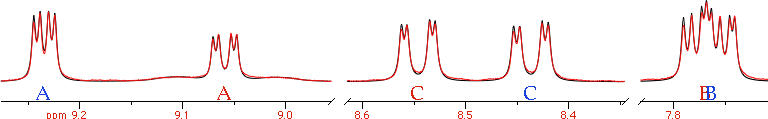
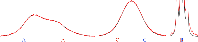
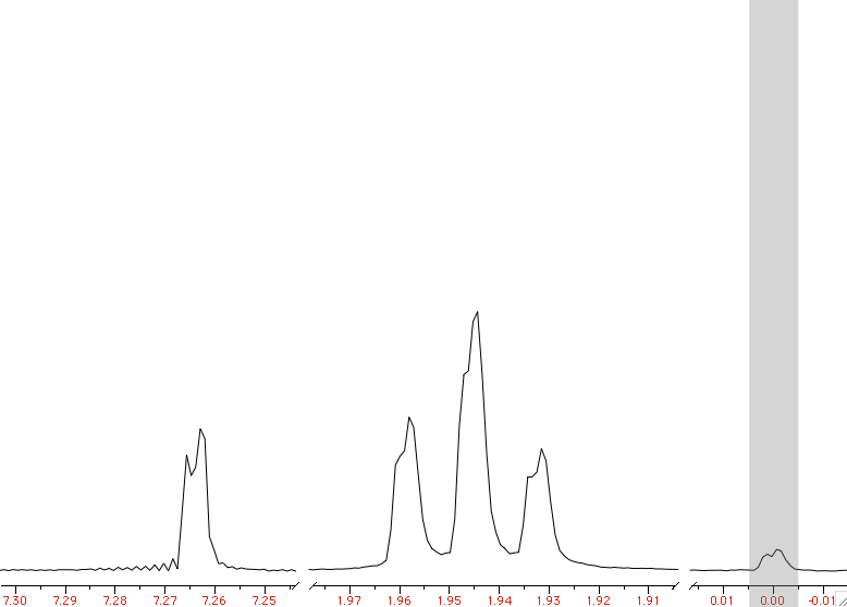
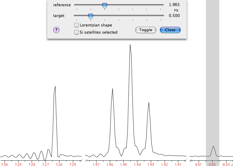
Manual AdjustmentThis can work if the spectrum, or portions of it, can be interpreted with first-order rules. Chemical shifts are easy to fit manually, because it's enough to literally drag each multiplet in place. The coupling constants can be adjusted in order, from the most evident (large) one to the most difficult (small) to extract. The process is simplified when the experimental multiplets are well resolved; in other words: apply a Lorentz-to-Gauss resolution enhancement by weighting the FID. Manual adjustment has become quite popular after the advent of interactive applications in the 90s. Don't dismiss it as "naive": it is certainly more accurate than extracting the coupling constants directly from the list of frequencies (which is an accepted and widespread practice). Visual fitting can be difficult with second-order spectra, but not for a skilled operator. The trick of the experts is to monitor the position of the weak combination lines. They are forbidden transitions that appear as tiny satellites. If you can simulate them exactly, the rest comes naturally in place. They are diagnostic, like canaries in a coal mine.
(2)
LaocoonThis was the name of the first popular program used to extract the Js from second-order, complicated multiplets. The program is no more in use today, but the method is still excellent. Quite simply it compares a list of experimental frequencies with a list of theoretical lines. Then improves the spectroscopic parameters according to the least squares principle. A lot of useful information is ignored, but this is also the strength of the method. When there is too much noise, or the baseline is problematic, or a solvent hides part of the spectrum, etc... you simply can't extract all the information from the spectrum, or you can but the intensities are not dependable. It's better to feed the algorithm with minimal selected data of high quality than hoping that a mass of errors can mutually compensate each other. With Laocoon it's not even necessary to match all the lines; as you can expect, the condition is that the number of parameters to guess must be less than the number of the lines. Despite the simplicity, this method requires more work, because you have to assign/match each experimental line to a theoretical line. This job looks trivial at the end of the process, because it's enough to match the lines in order of frequency. It's different when the starting guess is largely inaccurate. A single mismatch, in this case, is simple to discover, if you know the trick. The column of the residual errors will contain two large and opposite values. They correspond to the "swapped" lines. All considered, the most difficult part, for the user, is to read the manual of his/her program.
Here, more than in any other case, a Lorentz-to-Gauss weighting is beneficial: remember that you are not starting from the raw data points, but from the table of frequencies ("peak-picking"). It is
well known that the position of the maxima of a doublet doesn't coincide with the true line frequencies, when peaks are broad.

picture courtesy of the
nmr-analysis blog.
(3)
Total Line-shape (TLS)
I suspect that this approach derives, historically, from dynamic NMR, (the simulation of internal rotations, like in the case of DMF). You can, indeed, simulate a "static" system with a dynamic program, if the exchange rate is zero. DNMR (and the
programs that follow the same principle) don't recalculate the single lines (frequencies, intensities) but other sets of parameters that are used, eventually, to create the synthetic spectrum (plot). The latter can be compared, point by point, to the experiment, and the least squares are calculated from the difference. This is a great simplification for the user, compared to LAOCOON, because it's no more necessary to assign the lines. An higher quality of the experimental spectrum is however required, because the program now also employs the intensity information, and this information must be correct. Therefore the baseline must be flat and no extraneous peak can be present (it is trivial, however, to artificially delete isolated extraneous peaks/humps). Summarizing: you must spend time on processing the experimental spectrum.
We have seen that the first two methods prefer gaussian line-shapes.
This is not necessary with TLS, but we have the inverse problem: if you have already prepared the experimental spectrum for the other kinds of fit (with Gaussian shapes), can you perform a total lineshape fit? The answer is "NO" if we look at the original formulation of the method, but in practice it is possible, with some commercial package, to work with both kinds of shapes (and anything in between too).
Don't be mislead by the name "Total": nobody fits the whole spectrum, but only portions of it. Most of the tricks we learned when
fitting singlets (and collection of not-organized peaks) can be recycled with TLS. Actually, there is a minimal difference, from a mathematical point of view. In TLS, the algorithm varies a collection of parameters. They give a collection of lines, that are used to simulate the spectrum. In deconvolution, the algorithm directly start from the frequencies. That's the first difference. There is also a procedural difference: TLS has a built-in mechanism to escape from local minima. In practice, in the first stage of the fitting, a line broadening is applied that blurs the details. Once the multiplets has been set in the proper place, the broadening is removed and the details are taken into account. With plain line-fitting, there is no such need, because the first guess is extracted from the experimental spectrum itself, therefore everything is always in the right place (nearly).
If we called the previous method by the name of the first program implementing it, then TLS could be called, in a similar way, "DAVINS".